Neural Network, Transformer and GPT | Original
Table of Contents
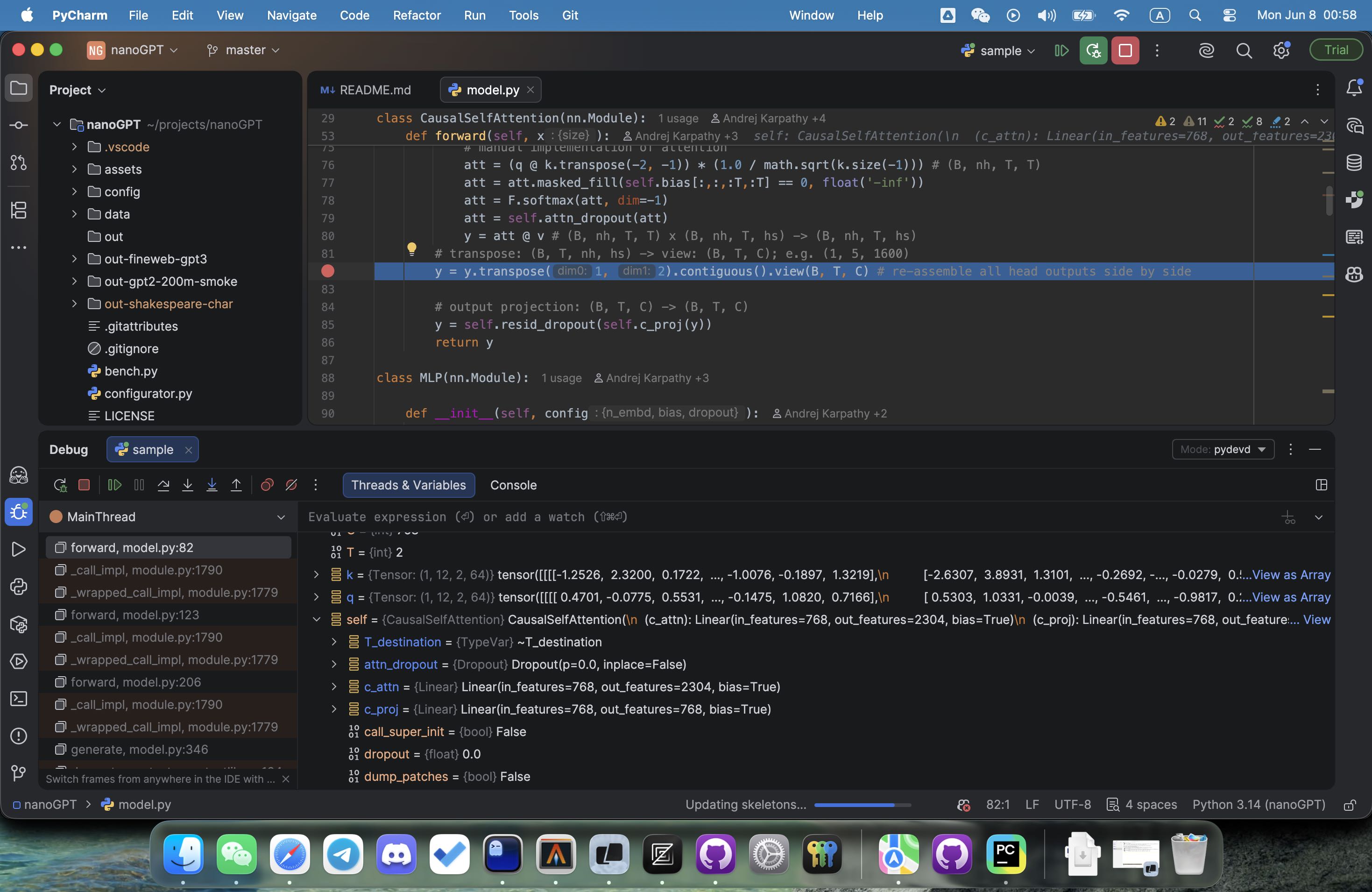
- AMD MI300X and Continued Transformer Learning
- Train GPT-2 on RTX 4070 and AMD MI300X
- Debugging in PyCharm
- How I Learned the KQV Mechanism in Transformers
- Query, Key, Value matrices represent token interactions
- Understanding requires knowing dimensions and shapes
- Initial concepts become clearer over time
- AI era provides abundant learning resources
- Inspiring stories motivate continued learning
- From Neural Network to GPT
- Replicate neural networks from scratch for understanding
- Transformers process text via embedding and encoding
- Self-attention calculates similarities between words
- Watch foundational lectures and read code
- Follow curiosity through projects and papers
- How Neural Network Works
- Backpropagation algorithm updates weights and biases
- Input data activates through network layers
- Feedforward computes layer outputs via sigmoid
- Error calculation guides learning adjustments
- Dimensional understanding is crucial for comprehension
AMD MI300X and Continued Transformer Learning
2026.06.08
-
Started training GPT-2 more extensively on the RTX 4070 and AMD MI300X.
-
Debugging the training pipeline in PyCharm.
How I Learned the KQV Mechanism in Transformers
2025.07.16
After reading K, Q, V Mechanism in Transformers, I somehow understood how K, Q, and V work.
Q stands for Query, K stands for Key, and V stands for Value. For a sentence, the Query is a matrix that stores the value of a token that it needs to ask other tokens about. The Key stands for the description of the tokens, and the Value stands for the actual meaning matrix of the tokens.
They have specific shapes, so one needs to know their dimensions and details.
I understood this around early June 2025. I first learned about it around the end of 2023. At that time, I read articles like The Illustrated Transformer, but I didn’t understand much.
After about two years, I found it easier to understand now. During these two years, I focused on backend work and preparing for my associate degree exams, and I didn’t read or learn much about machine learning. However, I did mull over these concepts from time to time when I was driving or doing other things.
This reminds me of the effect of time. We may learn a lot of things at first sight, even if we don’t comprehend much. But somehow, it triggers a starting point for our thinking.
Over time, I found that for knowledge and discovery, it is hard to think about or understand things the first time. But later, it seems easier to learn and know.
One reason is that in the AI era, it is easier to learn because you can delve into any detail or aspect to resolve your doubts. There are also more related AI videos available. More importantly, you see that so many people are learning and building projects on top of that, like llama.cpp.
The story of Georgi Gerganov is inspiring. As a new machine learning learner starting around 2021, he made a powerful impact in the AI community.
This kind of thing will happen again and again. So, for reinforcement learning and the latest AI knowledge, even though I am still not able to dedicate much time to them, I think I can find some time to quickly learn and try to think about them a lot. The brain will do its work.
From Neural Network to GPT
2023.09.28
YouTube Videos
Andrej Karpathy - Let’s build GPT: from scratch, in code, spelled out.
Umar Jamil - Attention is all you need (Transformer) - Model explanation (including math), Inference and Training
StatQuest with Josh Starmer - Transformer Neural Networks, ChatGPT’s foundation, Clearly Explained!!!
Pascal Poupart - CS480/680 Lecture 19: Attention and Transformer Networks
The A.I. Hacker - Michael Phi - Illustrated Guide to Transformers Neural Network: A step-by-step explanation
How I Learn
Once I had read half of the book “Neural Networks and Deep Learning”, I began to replicate the neural network example of recognizing handwritten digits. I created a repository on GitHub, https://github.com/lzwjava/neural-networks-and-zhiwei-learning.
That’s the real hard part. If one can write it from scratch without copying any code, one understands very well.
My replicate code still lacks the implementation of update_mini_batch and backprop. However, by carefully observing the variables in the phase of loading data, feed forwarding, and evaluating, I got a much better understanding of the vector, dimensionality, matrix, and shape of the objects.
And I began to learn the implementation of the GPT and transformer. By word embedding and positional encoding, the text changes to the numbers. Then, in essence, it has no difference to the simple neural network to recognize hand-written digits.
Andrej Karpathy’s lecture “Let’s build GPT” is very good. He explains things well.
The first reason is that it is really from scratch. We first see how to generate the text. It is kind of fuzzy and random. The second reason is that Andrej could say things very intuitively. Andrej did the project nanoGPT for several months.
I just had a new idea to judge the quality of the lecture. Can the author really write these codes? Why I don’t understand and which topic does the author miss? Besides these elegant diagrams and animations, what are their shortcomings and defects?
Back to the machine learning topic itself. As Andrej mentions, the dropout, the residual connection, the Self-Attention, the Multi-Head Attention, the Masked Attention.
By watching more above videos, I began to understand a bit.
By positional encoding with sin and cos functions, we get some weights. By word embedding, we change the words to numbers.
\[PE_{(pos,2i)} = sin(pos/10000^{2i/d_{model}}) \\ PE_{(pos,2i+1)} = cos(pos/10000^{2i/d_{model}})\]The pizza came out of the oven and it tasted good.
In this sentence, how does the algorithm know whether it refers to pizza or oven? How do we calculate the similarities for every word in the sentence?
We want a set of weights. If we use the transformer network to do the task of translation, every time we input a sentence, it can output the corresponding sentence of another language.
About the dot product here. One reason we use the dot product here is that the dot product will consider every number in the vector. What if we use the squared dot product? We first calculate the square of the numbers, then let them do the dot product. What if we do some reversed dot product?
About the masked here, we change the numbers of half of the matrix to the negative infinity. And then we use softmax to make the values range from 0 to 1. How about we change the left-bottom numbers to the negative infinity?
Plan
Continue to read code and papers and watch videos. Just have fun and follow my curiosity.
https://github.com/karpathy/nanoGPT
https://github.com/jadore801120/attention-is-all-you-need-pytorch
How Neural Network Works
2023.05.30
Let’s directly discuss the core of neural work. That said, the backpropagation algorithm:
- Input x: Set the corresponding activation \(a^{1}\) for the input layer.
- Feedforward: For each l=2,3,…,L compute \(z^{l} = w^l a^{l-1}+b^l\) and \(a^{l} = \sigma(z^{l})\)
- Output error \(\delta^{L}\): Compute the vector \(\delta^{L} = \nabla_a C \odot \sigma'(z^L)\)
- Backpropagate the error: For each l=L−1,L−2,…,2, compute \(\delta^{l} = ((w^{l+1})^T \delta^{l+1}) \odot \sigma'(z^{l})\)
- Output: The gradient of the cost function is given by \(\frac{\partial C}{\partial w^l_{jk}} = a^{l-1}_k \delta^l_j\) and \(\frac{\partial C}{\partial b^l_j} = \delta^l_j\)
This is copied from Michael Nelson’s book Neural Networks and Deep Learning. Is it overwhelming? It might be at the first time you see it. But it is not after one month of studying around it. Let me explain.
Input
There are 5 phases. The first phase is Input. Here we use handwritten digits as input. Our task is to recognize them. One handwritten digit has 784 pixels, which is 28*28. In every pixel, there is a grayscale value which is range from 0 to 255. So the activation means that we use some function to activate it, to change its original value to a new value for the convenience of processing.
Say, we have now 1000 pictures of 784 pixels. We now train it to recognize what digit they show. We have now 100 pictures to test that learning effect. If the program can recognize 97 pictures’ digits, we say its accuracy is 97%.
So we would loop over the 1000 pictures, to train out the weights and biases. We make weights and biases more correct every time we give it a new picture to learn.
One batch training result is to be reflected in 10 neurons. Here, the 10 neurons represent from 0 to 9 and its value is range from 0 to 1 to indicate how their confidence about its accuracy.
And the input is 784 neurons. How can we reduce 784 neurons to 10 neurons? Here is the thing. Let’s suppose we have two layers. What does the layer mean? That is the first layer, we have 784 neurons. In the second layer, we have 10 neurons.
We give each neuron in the 784 neurons a weight, say,
\[w_1, w_2, w_3, w_4, ... , w_{784}\]And give the first layer, a bias, that is, \(b_1\).
And so for the first neuron in the second layer, its value is:
\[w_1*a_1 + w_2*a_2+...+ w_{784}*a_{784}+b_1\]But these weights and a bias are for \(neuron^2_{1}\)(the first one in the second layer). To the \(neuron^2_{2}\), we need another set of weights and a bias.
How about the sigmoid function? We use the sigmoid function to map the value of the above from 0 to 1.
\[\begin{eqnarray} \sigma(z) \equiv \frac{1}{1+e^{-z}} \end{eqnarray}\] \[\begin{eqnarray} \frac{1}{1+\exp(-\sum_j w_j x_j-b)} \end{eqnarray}\]We also use the sigmoid function to activate the first layer. That said, we change that grayscale value to the range from 0 to 1. So now, every neuron in every layer has a value from 0 to 1.
So now for our two-layer network, the first layer has 784 neurons, and the second layer has 10 neurons. We train it to get the weights and biases.
We have 784 * 10 weights and 10 biases. In the second layer, for every neuron, we will use 784 weights and 1 biases to calculate its value. The code here like,
    def __init__(self, sizes):
        self.num_layers = len(sizes)
        self.sizes = sizes
        self.biases = [np.random.randn(y, 1) for y in sizes[1:]]
        self.weights = [np.random.randn(y, x)
                        for x, y in zip(sizes[:-1], sizes[1:])]
Feedforward
Feedforward: For each l=2,3,…,L compute \(z^{l} = w^l a^{l-1}+b^l\) and \(a^{l} = \sigma(z^{l})\)
Notice here, we use the value of the last layer, that is \(a^{l-1}\) and the current layer’s weight, \(w^l\) and its bias \(b^l\) to do the sigmoid to get the value of the current layer, \(a^{l}\).
Code:
        nabla_b = [np.zeros(b.shape) for b in self.biases]
        nabla_w = [np.zeros(w.shape) for w in self.weights]
        # feedforward
        activation = x
        activations = [x]
        zs = []
        for b, w in zip(self.biases, self.weights):
            z = np.dot(w, activation)+b
            zs.append(z)
            activation = sigmoid(z)
            activations.append(activation)
Output error
Output error \(\delta^{L}\): Compute the vector \(\delta^{L} = \nabla_a C \odot \sigma'(z^L)\)
Let’s see what the \(\nabla\) mean.
\[\begin{eqnarray} w_k & \rightarrow & w_k' = w_k-\eta \frac{\partial C}{\partial w_k} \\ b_l & \rightarrow & b_l' = b_l-\eta \frac{\partial C}{\partial b_l} \end{eqnarray}\]Del, or nabla, is an operator used in mathematics (particularly in vector calculus) as a vector differential operator, usually represented by the nabla symbol ∇.
Here \(\eta\) is the learning rate. We use the derivative that C is respective to the weights and the bias, that is the rate change between them. That is sigmoid_prime in the below.
Code:
        delta = self.cost_derivative(activations[-1], y) * \
            sigmoid_prime(zs[-1])
        nabla_b[-1] = delta
        nabla_w[-1] = np.dot(delta, activations[-2].transpose())
    def cost_derivative(self, output_activations, y):
        return (output_activations-y)
Backpropagate the error
Backpropagate the error: For each l=L−1,L−2,…,2, compute \(\delta^{l} = ((w^{l+1})^T \delta^{l+1}) \odot \sigma'(z^{l})\)
     for l in range(2, self.num_layers):
            z = zs[-l]
            sp = sigmoid_prime(z)
            delta = np.dot(self.weights[-l+1].transpose(), delta) * sp
            nabla_b[-l] = delta
            nabla_w[-l] = np.dot(delta, activations[-l-1].transpose())
        return (nabla_b, nabla_w)
Output
Output: The gradient of the cost function is given by \(\frac{\partial C}{\partial w^l_{jk}} = a^{l-1}_k \delta^l_j\) and \(\frac{\partial C}{\partial b^l_j} = \delta^l_j\)
    def update_mini_batch(self, mini_batch, eta):
        nabla_b = [np.zeros(b.shape) for b in self.biases]
        nabla_w = [np.zeros(w.shape) for w in self.weights]
        for x, y in mini_batch:
            delta_nabla_b, delta_nabla_w = self.backprop(x, y)
            nabla_b = [nb+dnb for nb, dnb in zip(nabla_b, delta_nabla_b)]
            nabla_w = [nw+dnw for nw, dnw in zip(nabla_w, delta_nabla_w)]
        self.weights = [w-(eta/len(mini_batch))*nw
                        for w, nw in zip(self.weights, nabla_w)]
        self.biases = [b-(eta/len(mini_batch))*nb
                       for b, nb in zip(self.biases, nabla_b)]
Final
It is a short article. And in the most part, it just shows the code and math formula. But it is fine to me. Before writing it, I don’t understand clearly. After writing or just copying snippets from code and book, I understand most of it. After gaining confidence from the teacher Yin Wang, reading about 30% of the book Neural Networks and Deep Learning, listening to the Andrej Karpathy’s Standford lectures and Andrew Ng’s courses, discussing with my friend Qi, and tweaking with Anaconda, numpy, and Theano libraries to make the code years ago work, I now understand it.
One of the key points is the dimensions. We should know the dimensions of every symbol and variable. And it just does the differentiable computation. Let’s end with Yin Wang’s quotes:
Machine learning is really useful, one might even say beautiful theory, because it is simply calculus after a makeover! It is the old and great theory of Newton, Leibniz, in a simpler, elegant and powerful form. Machine learning is basically the use of calculus to derive and fit some functions, and deep learning is the fitting of more complex functions.
There is no ‘intelligence’ in artificial intelligence, no ‘neural’ in neural network, no ‘learning’ in machine learning, and no ‘depth’ in deep learning. There is no ‘depth’ in deep learning. What really works in this field is called ‘calculus’. So I prefer to call this field ‘differentiable computing’, and the process of building models is called ‘differentiable programming’.
Original. Curating and sharing still takes effort.
If you find it useful, feel free to
donate.
WeChat: @lzwjava ·
X: @lzwjava ·
Say hi 👋
·
X: @lzwjava ·
Say hi 👋