Zen and the Art of Machine Learning

Home

---

Zen

A young dad is busy learning Neural networks at the weekend. However, this weekend, he needed to accompany his baby daughter to swim in the pool of the apartment complex. He laid down in the shallow water and watched the top apartment buildings rising top to the sky. And suddenly he thought, Wow, they are a lot like neural networks. Every balcony is just like a neuron. And a building is like a layer of neurons. And a group of buildings are combined to be a neural network.

He then thought about backpropagation. What backpropagation does is to backpropagate the errors to neurons. At the end of one-time training, the algorithm calculates the error between the output of the last layer to the target result. Actually, neural networks have nothing to do with neurons. It is about differentiable computing.

After writing down the article “I Finally Understand How Neural Network Works”, he found that he still didn’t understand. Understanding is a relative thing. As Richard Feynman points out something like nobody can be 100% sure about anything, we can only be relatively sure about something. So it is acceptable for Zhiwei to say so.

So he figured out a way to understand the Neural Networks deeply by using the way to copy several lines of example code every time, then run it and print variables. It is about the simple neural network to recognize the handwritten digits. The book he is reading recently is titled Neural Networks and Deep Learning. So he gives his GitHub repository the name Neural Networks and Zhiwei Learning.

Before we use Neural Network to train our data, we need to load data first. This part costs him a week of leisure time to do it. Things are always needed more time to get them done. But as long as we don’t give up, we are capable to do pretty many things.

The mnist in the Machine learning area stands for Modified National Institute of Standards and Technology database. So our data loader file is called minst_loader. We use the print function in Python to print a lot of lists and arrays of ndarray. The nd in ndarray means n-dimensional.

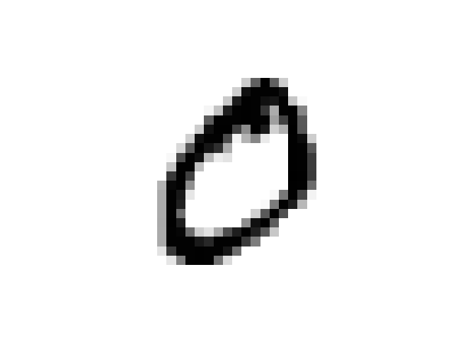
Besides print, we must use the matplotlib library to show our digits. Like below.

Art

Let’s see more digits.

(Image source: Neural Networks and Deep Learning)

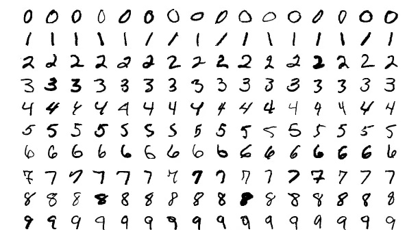
It is more joyful when you sometimes can see pictures instead of facing around the noisy codes all day long.

(Image source: Neural Networks and Deep Learning)

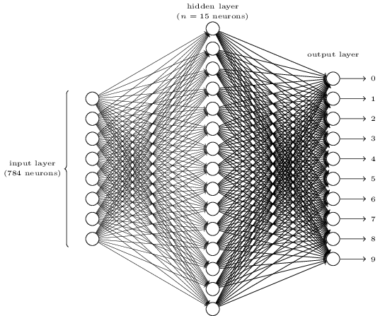
Does it seem complicated? Here, we may have too many neurons in each layer. And it makes things obscure. It is actually very simple once you understood it. First thing about the above picture is that it has three layers, the input layer, the hidden layer and the output layer. And one layer connects the next layer. But how can 784 neurons in the input layer change to the 15 neurons in the second layer? And how can 15 neurons in the hidden layer change to the 10 neurons in the output layer?

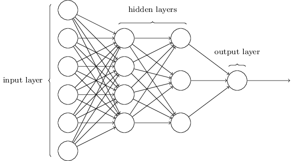
This network is much simpler. Though Zhiwei doesn’t want to include any math formula in this article, here the math is too simple and beautiful to hide.

\[w_1*a_1 + w_2*a_2+...+ w_6*a_6+b_1\]

Suppose we indicate the network like below.

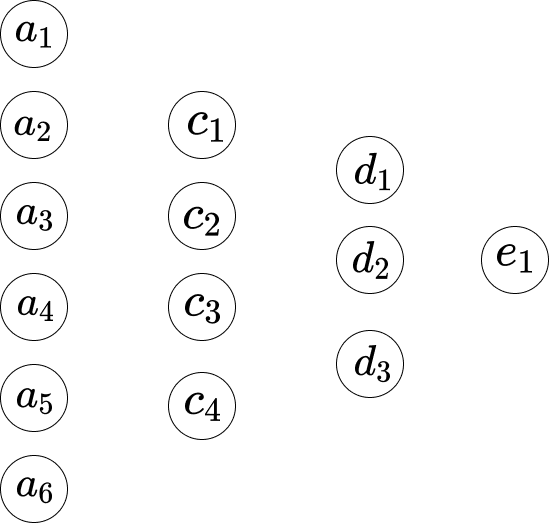
So between the first layer and the second layer, we have the below equations.

\[\begin{eqnarray} w_1*a_1 +...+ w_6*a_6+b_1 = c_1 \\ w_1*a_1 +...+ w_6*a_6+b_2 = c_2 \\ w_1*a_1 +...+ w_6*a_6+b_3 = c_3 \\ w_1*a_1 +...+ w_6*a_6+b_4 = c_4 \end{eqnarray}\]

Here, Equation 1 has a group set of weights, Equation 2 has another group set of weights. So the $w_1$ in Equation 1 is different from the $w_1$ in Equation 2. And so between the second layer and the third layer, we have the below equations.

\[\begin{eqnarray} w_1*c_1 + ... + w_4*c_4+b_1 = d_1 \\ w_1*c_1 + ... + w_4*c_4+b_2 = d_2 \\ w_1*c_1 + ... + w_4*c_4+b_3 = d_3 \end{eqnarray}\]

And in the third layer to the last layer, we have the below equations.

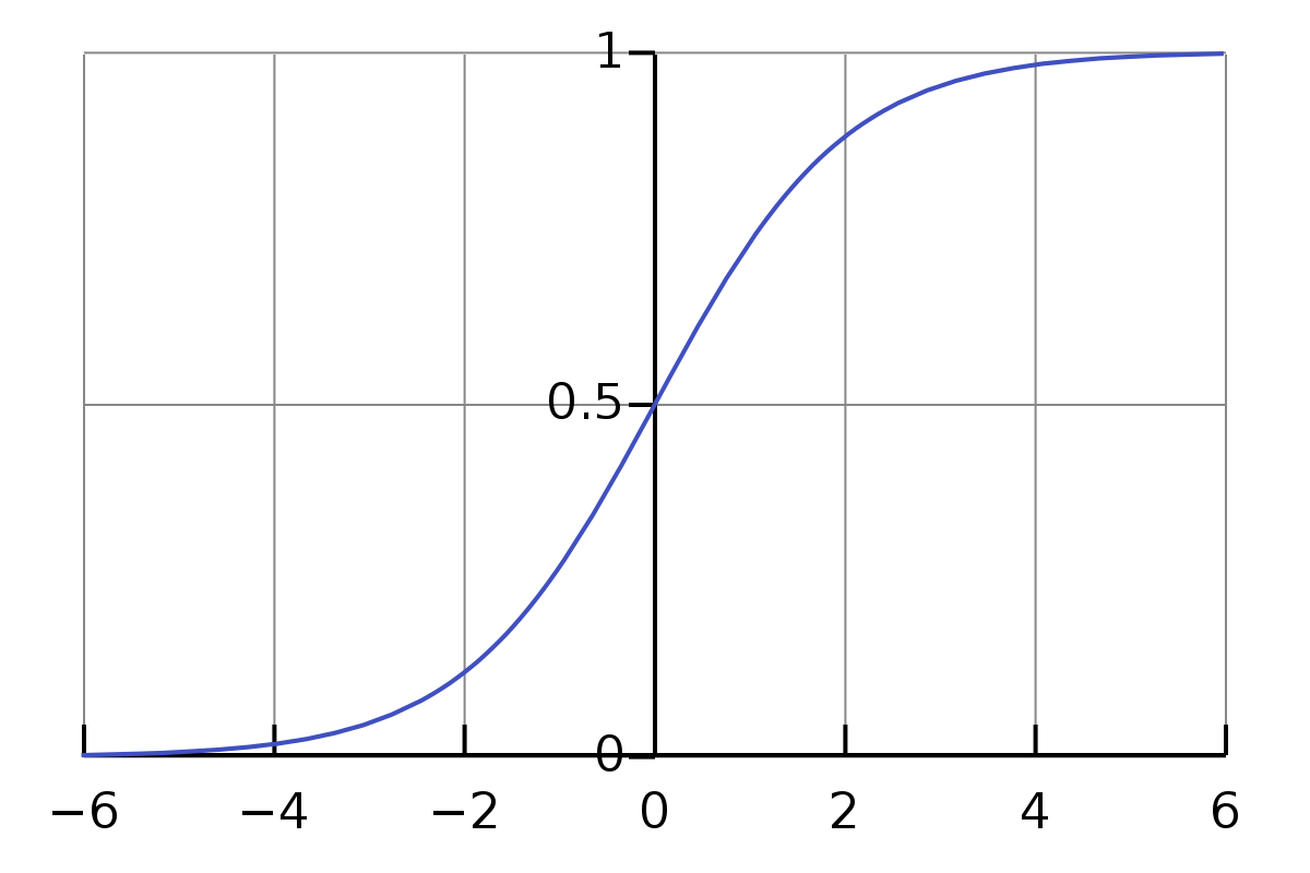
\[w_1*d_1 + w_2*d_2+ w_3*d_3+ b_1 = e_1\]

The one problem with the above equations is that the value is not simple or formal enough. The range of the value of multiplication and addition is quite large. We want it constrained in a small range, say, 0 to 1. So here, we have the Sigmoid function.

\[\sigma(z) \equiv \frac{1}{1+e^{-z}}\]

We don’t need to be intimidated by the sigma symbol $\sigma$. It is just a symbol just like the symbol a. If we give it the input as 0.5, its value is

\[\frac{1}{1+e^{-0.5}} \approx 0.622459\]

And,

\[\begin{eqnarray} \frac{1}{1+e^{-(-100)}} \approx 3.72*e^{-44} \\ \frac{1}{1+e^{-(-10)}} \approx 0.000045 \\ \frac{1}{1+e^{-(-1)}} \approx 0.26894 \\ \frac{1}{1+e^{-{0}}} = 0.5 \\ \frac{1}{1+e^{-10}} \approx 0.99995 \\ \frac{1}{1+e^{-100}} = 1 \end{eqnarray}\]

It is intriguing here. I don’t know the above before I write this article. Now, I got a feeling about how its approximate result value for the normal input. And we observe that for the input that ranges from 0 to $\infty$, its value is from 0.5 to 1, and for the input that ranges from $-\infty$ to 0, its value is from 0 to 0.5.

So regarding the above equations, they are not accurate. The most proper ones should be like below.

\[\begin{eqnarray} \sigma(w_1*a_1 + ... + w_6*a_6+b_1) = c_1 \\ \sigma(w_1*a_1 + ... + w_6*a_6+b_2) = c_2 \\ \sigma(w_1*a_1 + ... + w_6*a_6+b_3) = c_3 \\ \sigma(w_1*a_1 + ... + w_6*a_6+b_4) = c_4 \end{eqnarray}\]

So for the first equation, it is that,

\[\frac{1}{1+e^{-(w_1*a_1 +...+ w_6*a_6+b_1)}}\]

How can we update the new weight for $w_1$? That is,

\[w_1 \rightarrow w_1' = w_1- \Delta w\]

To the equation,

\[w_1*a_1 + w_2*a_2+...+ w_6*a_6+b_1\]

Its derivative to the $w_1$ is $a_1$. Let’s give the sum a symbol $S_1$.

So,

\[\frac{\partial S_1}{\partial w_1} = a_1 , \frac{\partial S_1}{\partial w_2} = a_2, ...\]

The derivate means the rate of change. It means that for the change $\Delta w$ in $w_1$, its change in the result $S_1$ is $a_1 * \Delta w$. And how can we reverse such a calculation? Let’s calculate it.

\[\begin{eqnarray} S_1' - S_1 = \Delta S_1 \\ \frac{\Delta S_1}{a_1} = \Delta w \\ w_1- \Delta w = w_1' \end{eqnarray}\]

And the chain rule explains that the derivative of $f(g(x))$ is $f’(g(x))⋅g’(x)$.

So here,

\[\begin{eqnarray} f(z) = \sigma(z) = \frac{1}{1+e^{-z}} \\ g(x) = w_1*a_1 +...+ w_6*a_6+b_1 \end{eqnarray}\]

And the derivative of the sigmoid function is,

\[\sigma'(z) = \frac{\sigma(z)}{1-\sigma(z)}\]

So the derivative of $f(g(w_1))$ is $\frac{\sigma(z)}{1-\sigma(z)} * a_1$.

So,

\[\begin{eqnarray} \frac{\sigma(z)}{1-\sigma(z)} * a_1 * \Delta w = \Delta C \\ \Delta w = \frac{\Delta C}{\frac{\sigma(z)}{1-\sigma(z)} * a_1} \end{eqnarray}\]

And for the bias $b_1$,

\[\begin{eqnarray} g'(b_1) = 1 \\ \frac{\sigma(z)}{1-\sigma(z)} * \Delta b = \Delta C \\ \Delta b = \frac{\Delta C}{\frac{\sigma(z)}{1-\sigma(z)}} \end{eqnarray}\]

Code

The way of printing variables is very useful and simple, though nowadays people invent Jupyter Notebook to do such things. As Zhiwei mentions before, one of the keys to understanding neural networks is that we should pay attention to the dimensions.

def print_shape(array):
    arr = np.array(array)
    print(arr.shape)
    
print(len(test_data[0][0])) # 10
print_shape(training_results[0]) # (784, 1)
print(list(training_data)[0:1]) # <class 'list'>

As now Zhiwei just finished the loading data part, he will continue to use the same way of copying several lines and printing variables to learn the actual part of the neural network. You may follow the progress here, https://github.com/lzwjava/neural-networks-and-zhiwei-learning.

I got stuck several times in the progress. Even though it seems very simple code, after one time by one time trying to understand it, I failed. And then I moved myself out of the current line of the code to look at it from a high level, to think about why the author writes that part of the code, then suddenly I got it. The code is below.

def load_data_wrapper():
    tr_d, va_d, te_d = load_data()

    training_inputs = [np.reshape(x, (784, 1)) for x in tr_d[0]]
    training_results = [vectorized_result(y) for y in tr_d[1]]
    training_data = zip(training_inputs, training_results)

    validation_inputs = [np.reshape(x, (784, 1)) for x in va_d[0]]
    validation_data = zip(validation_inputs, va_d[1])

    test_inputs = [np.reshape(x, (784, 1)) for x in te_d[0]]
    test_data = zip(test_inputs, te_d[1])
    return (training_data, validation_data, test_data)

def vectorized_result(j):
    e = np.zeros((10, 1))
    e[j] = 1.0
    return e    

Here, the dimensions of the variables are complex. However, when we think about the initiative of the author, then we have some clues. Look at it, the code is composite with three similar parts. And every part is almost the same though the names of variables are different. Now, it seems very comfortable to me. The zip, the “for” operation to the list, and the reshape function. The understanding just accumulates between the hundreds of times of printing variables and trying to figure out why the values of the variables be so.

And Zhiwei always finds errors very valuable. Like the below code, he faces a lot of errors, for example,

• TypeError: Invalid shape (784,) for image data
• ValueError: setting an array element with a sequence. The requested array has an inhomogeneous shape after 2 dimensions. The detected shape was (1, 2) + inhomogeneous part.

The error stack trace is just like a beautiful poem.

Also, when we format the value output in Visual Studio Code, it is much more readable.

[array([[0.92733598],
       [0.01054299],
       [1.0195613],
       ...
       [0.67045368],
       [-0.29942482],
       [-0.35010666]]),
 array([[-1.87093344],
        [-0.18758503],
        [1.35792778],
        ...
        [0.36830578],
        [0.61671649],
        [0.67084213]])]

読んでくれてありがとう. Thank you for your reading.

---

Note: Some pictures are copied from the book “Neural Networks and Deep Learning”.

---

Back